How to create a Thermometer Chart in Excel

Download PC Repair Tool to quickly find & fix Windows errors automatically

A Thermometer chart looks like a thermometer. The Thermometer chart is a keen way to represent data in Microsoft Excel when y'all have an bodily value and a target value and excellent to clarify sales functioning.

Does Excel take a Thermometer nautical chart?

The Thermometer chart is not a default nautical chart in Excel or whatever Office programs; y'all have to create one from scratch. In this tutorial, we will explain how to create a thermometer chart in Microsoft Excel.

How to create a Thermometer Chart in Excel

Follow the steps below to create a thermometer nautical chart in Excel.

Launch Excel.
Enter information into the Excel spreadsheet.
Select the achieve and target data
Click the Insert tab
Click the Column button in the Charts group and select the Stacked cavalcade from the drib-down menu.
A Chart Design tab will appear; click information technology.
On the Chart Blueprint tab, click the Switch the Row and Column push button.
Right-click the Orange serial and select Format Data Series from the context menu.
A Format Data Serial pane will appear.
Drag the Gap width to zero
Click the fill up section and click No Fill.
Click the Border section and click Solid Line.
And so select the color yous desire from the Color drop-down menu.
Under the border section, input ane.5 pt in the Width box.
At present resize the chart.
Remove the Nautical chart title.
And so go to the Format tab and select the Oval shape from the Insert Shapes group.
Depict the oval shape at the bottom of the chart.
Click the Shape Outline button and select a color that matches the color in your chart.
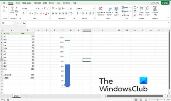
Now, we accept a Thermometer chart.

Launch Excel.

Enter information into the Excel spreadsheet.

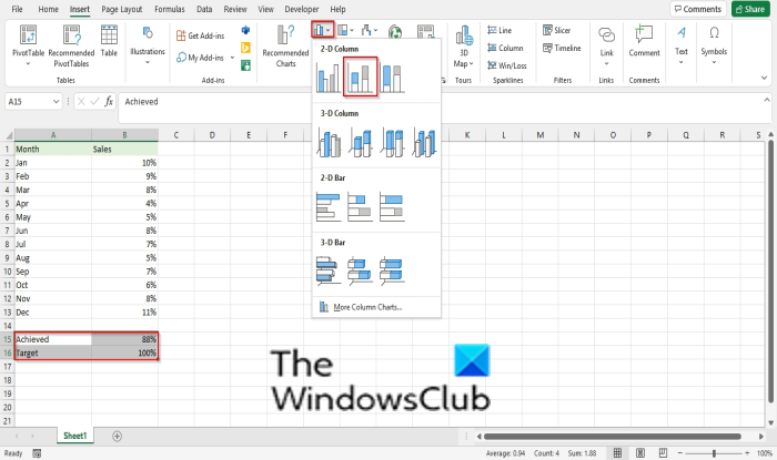
Select the reach and target data

Click the Insert tab

Click the Column push in the Charts group and select the Stacked cavalcade from the drop-down menu.

A Chart Design tab volition appear; click it.

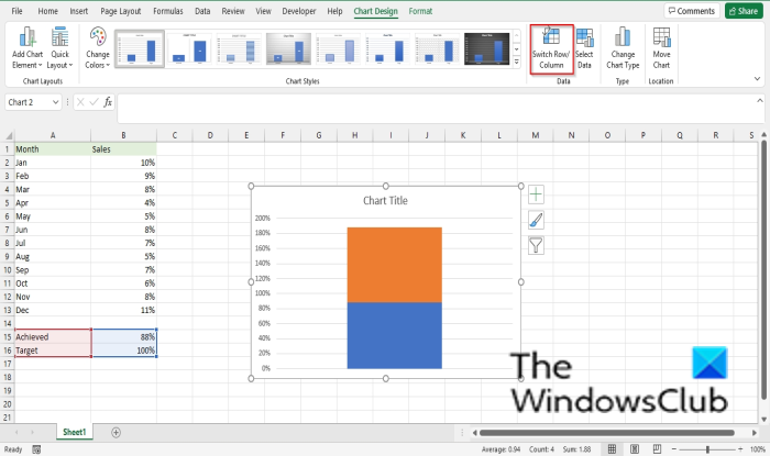
On the Nautical chart Pattern tab, click the Switch the Row and Column button.

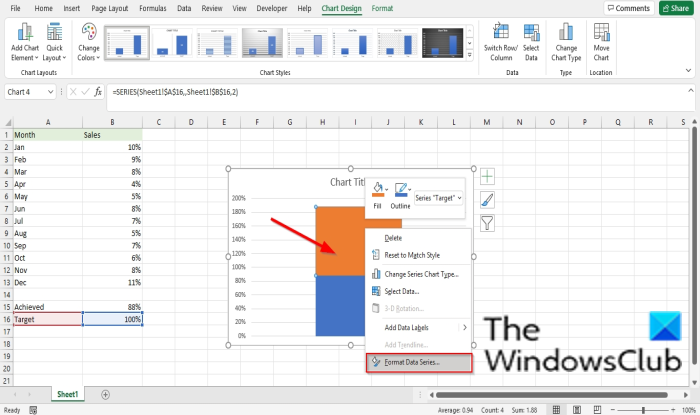
Right-click the Orange series and select Format Data Series from the context menu.

A Format Information Series pane volition appear.

Drag the Gap width to zero.

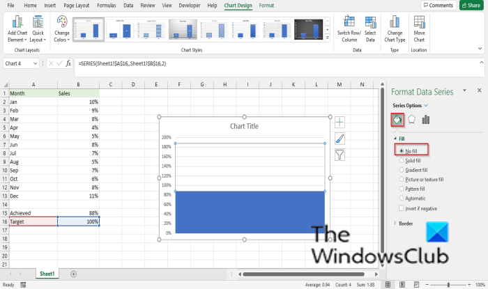
Click the Fill department and click No Fill.

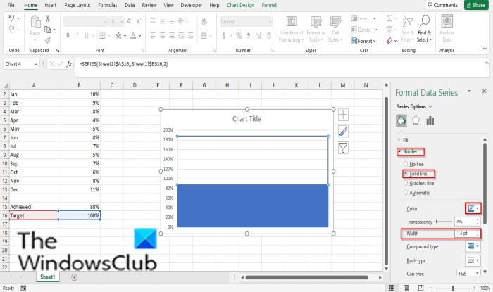
Click the Edge section and click Solid Line.

Then select the color you desire from the Color drib-down menu.

Under the edge section, input one.5 pt in the Width box.

Now resize the chart.

Remove the Nautical chart title.

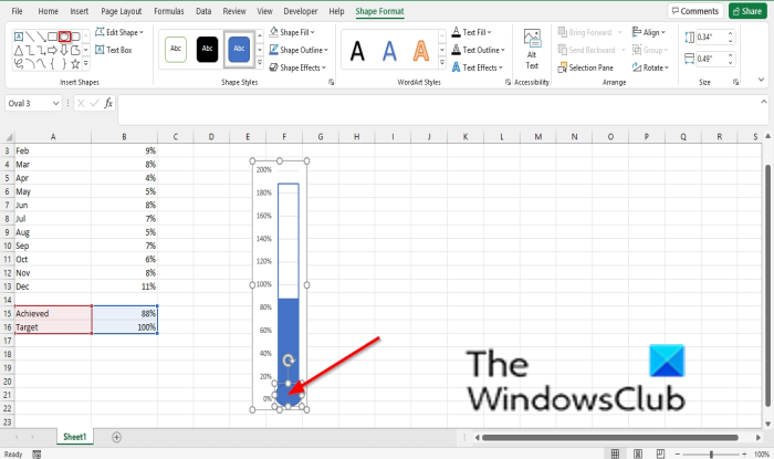
Then go to theFormat tab and select the Oval shape from the Insert Shapes group.

Draw the oval shape at the lesser of the nautical chart.

Click the Shape Make full button and select a color that matches the color in your chart.

Now, nosotros have a Thermometer nautical chart.

Read: How to alter default browser when opening hyperlinks in Excel.

We hope this tutorial helps you understand how to create a Thermometer Chart in Excel; if you have questions virtually the tutorial, let us know in the comments.

Shantel is a university educatee studying for Bachelor of Science in Information Engineering science. Her goal is to become a Database Administrator or a Organisation Administrator. She enjoys reading and watching historical documentaries and dramas.